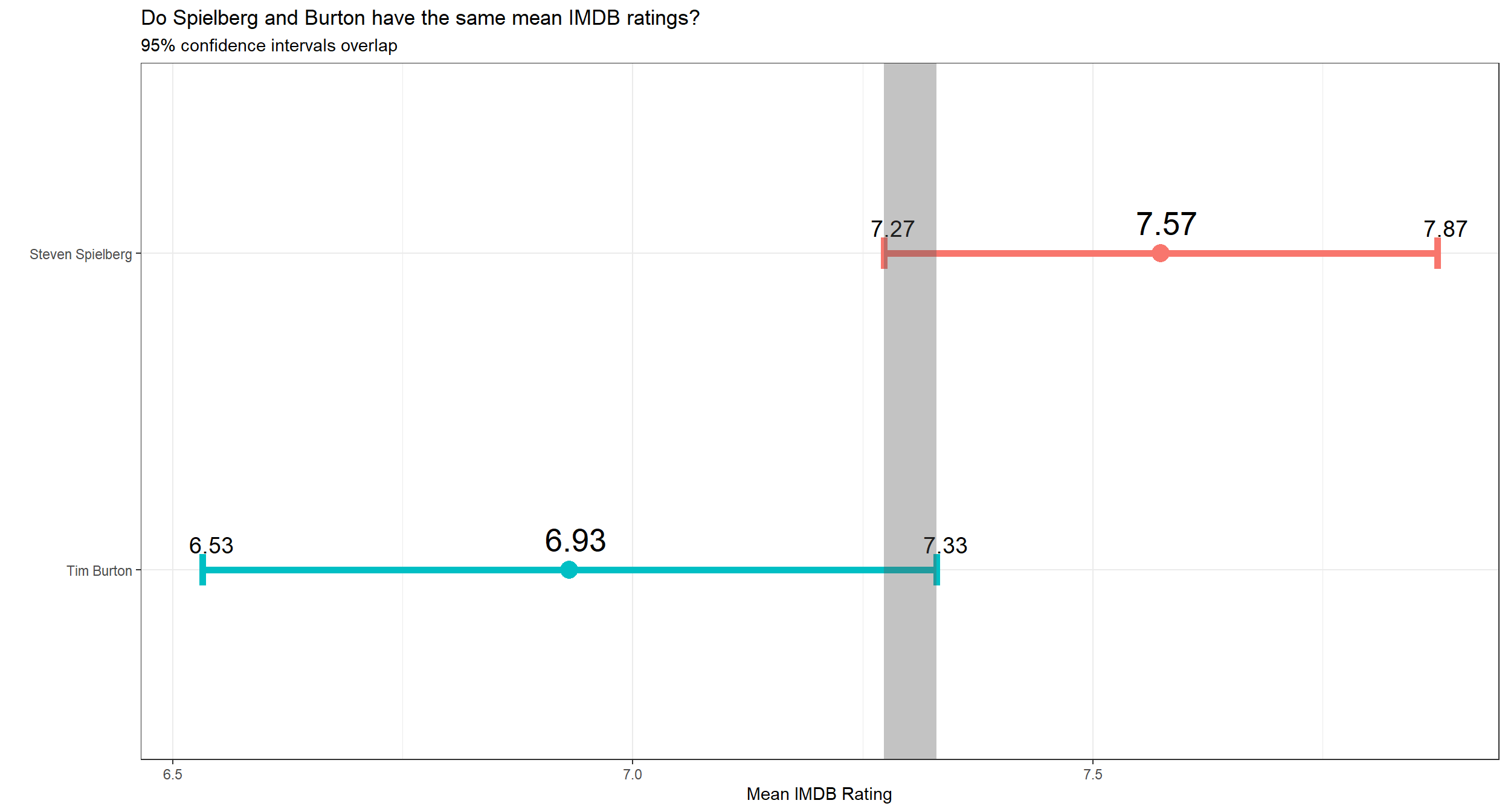
Replicating plot of confidence intervals for the mean ratings of the two directors

movies <- read_csv(here::here("data", "movies.csv"))
glimpse(movies)

## Rows: 2,961
## Columns: 11
## $ title               <chr> "Avatar", "Titanic", "Jurassic World", "The Ave...
## $ genre               <chr> "Action", "Drama", "Action", "Action", "Action"...
## $ director            <chr> "James Cameron", "James Cameron", "Colin Trevor...
## $ year                <dbl> 2009, 1997, 2015, 2012, 2008, 1999, 1977, 2015,...
## $ duration            <dbl> 178, 194, 124, 173, 152, 136, 125, 141, 164, 93...
## $ gross               <dbl> 7.61e+08, 6.59e+08, 6.52e+08, 6.23e+08, 5.33e+0...
## $ budget              <dbl> 2.37e+08, 2.00e+08, 1.50e+08, 2.20e+08, 1.85e+0...
## $ cast_facebook_likes <dbl> 4834, 45223, 8458, 87697, 57802, 37723, 13485, ...
## $ votes               <dbl> 886204, 793059, 418214, 995415, 1676169, 534658...
## $ reviews             <dbl> 3777, 2843, 1934, 2425, 5312, 3917, 1752, 1752,...
## $ rating              <dbl> 7.9, 7.7, 7.0, 8.1, 9.0, 6.5, 8.7, 7.5, 8.5, 7....

#loading data
movies <- read_csv(here::here("data", "movies.csv"))


#calculating the CIs
Two_directors <- movies %>% 
  group_by(director) %>% 
  filter(director %in% c("Tim Burton", "Steven Spielberg")) %>% 
  summarise(average_rating = mean(rating), 
            SD_rating = sd(rating), 
            count = n(), 
            t_critical = qt(0.975, count - 1),
            SE =  SD_rating/sqrt(count),  
            margin_of_error = t_critical * SE, 
            ci_low = average_rating - margin_of_error,  
            ci_high = average_rating + margin_of_error) 

#displaying statistics
Two_directors

## # A tibble: 2 x 9
##   director average_rating SD_rating count t_critical    SE margin_of_error
##   <chr>             <dbl>     <dbl> <int>      <dbl> <dbl>           <dbl>
## 1 Steven ~           7.57     0.695    23       2.07 0.145           0.301
## 2 Tim Bur~           6.93     0.749    16       2.13 0.187           0.399
## # ... with 2 more variables: ci_low <dbl>, ci_high <dbl>

#overlaps
xmin_rect = Two_directors %>% 
  filter(director == "Steven Spielberg") %>% 
  select(ci_low)

xmax_rect = Two_directors %>% 
  filter(director == "Tim Burton") %>% 
  select(ci_high)

#plotting
ggplot(Two_directors, aes(y=factor(director, levels = c("Tim Burton", "Steven Spielberg")), 
  x = average_rating, group = director)) +
  geom_point(aes(color=director), size = 5) +
  geom_errorbar(aes(xmin=ci_low, xmax=ci_high, color=director), width=.1, size = 2) +
  geom_text(aes(label = round(ci_low,2), x = ci_low),
            hjust = 0.3, 
            vjust = -1, 
            size = 5) + 
  geom_text(aes(label = round(ci_high,2), x = ci_high), 
            hjust = 0.3, 
            vjust = -1, 
            size = 5) +
  geom_text(aes(label = round(average_rating,2), x = average_rating), 
            hjust = 0.4, 
            vjust = -0.8, 
            size = 7) + 
  geom_rect(aes(xmin = xmin_rect$ci_low, xmax = xmax_rect$ci_high, ymin = -Inf, ymax = Inf), alpha = 0.2) +
  theme_bw() +
  theme(legend.position = "none") +
  labs(title = "Do Spielberg and Burton have the same mean IMDB ratings?",
       subtitle = "95% confidence intervals overlap",
       y = "",
       x = "Mean IMDB Rating")

T test and Hypothesis test

T_test <- movies %>%
  select(director, rating) %>%
  filter(director == "Steven Spielberg" | director == "Tim Burton")

t.test(rating ~ director, data =T_test)

## 
##  Welch Two Sample t-test
## 
## data:  rating by director
## t = 3, df = 31, p-value = 0.01
## alternative hypothesis: true difference in means is not equal to 0
## 95 percent confidence interval:
##  0.16 1.13
## sample estimates:
## mean in group Steven Spielberg       mean in group Tim Burton 
##                           7.57                           6.93

Bases on the p-value of 0.01 which is less than 0.05, we reject the null hypothesis and assume that the average IMDB Ratings for Steven Spielberg and Tim Burton are not the same.

#calculating the differences in means
differences<- T_test%>%
specify(rating ~ director)%>%
calculate(stat="diff in means",order=c("Steven Spielberg","Tim Burton")) 

#simulating the null distribution
null_dist<-T_test%>%
specify(rating ~ director)%>%
hypothesize(null="independence")%>%
generate(reps=1000,type="permute")%>%
calculate(stat="diff in means",order=c("Steven Spielberg","Tim Burton"))

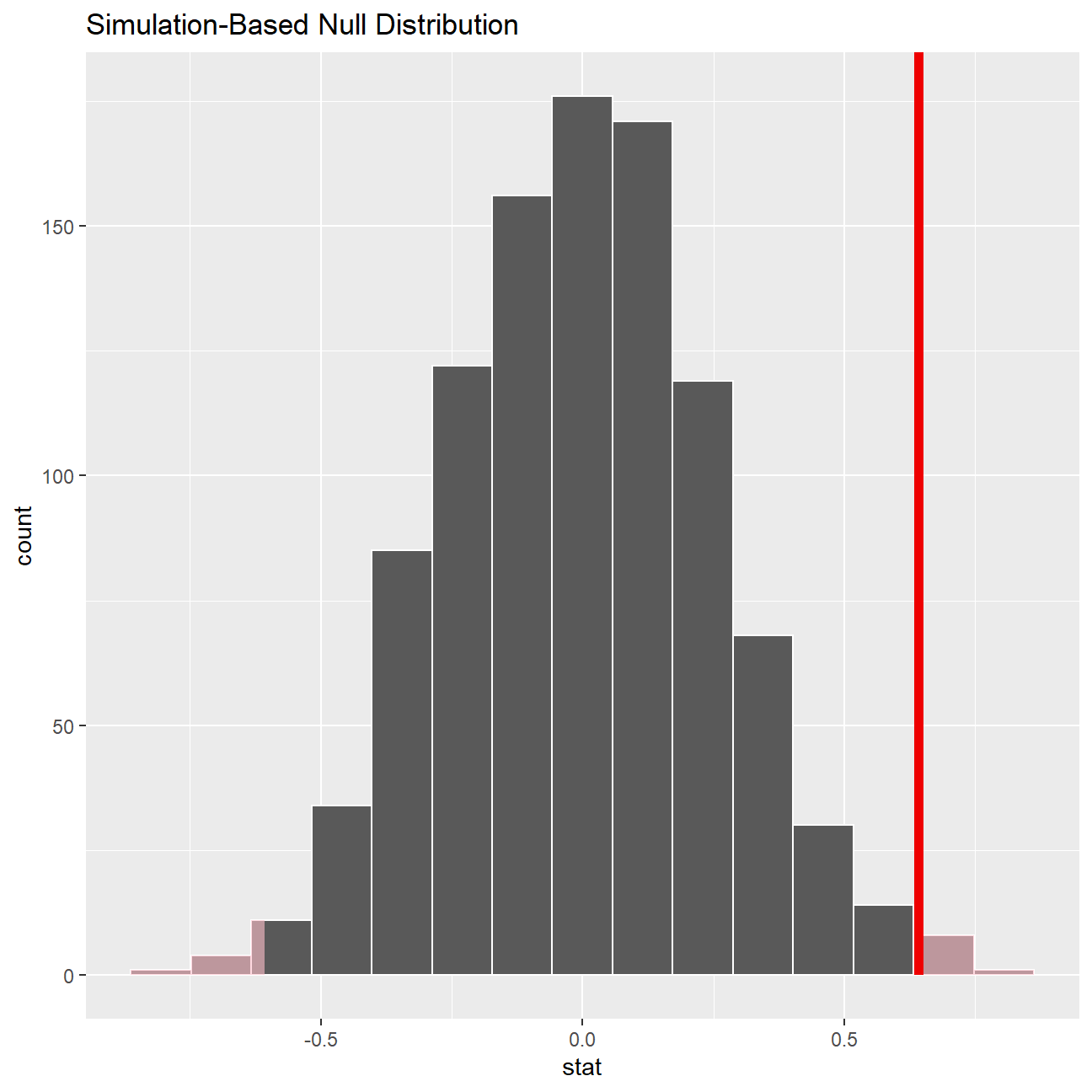
#Visualising null distibtution and p-value
null_dist %>% 
visualise() +
  shade_p_value(obs_stat = differences, direction = "two-sided") 

null_dist %>% get_p_value(obs_stat = differences, direction = "two_sided")

## # A tibble: 1 x 1
##   p_value
##     <dbl>
## 1   0.018

After running the test several times the p-value for the simulation based test was usually between 0.01 and 0.024, which is very close the one for our traditional test. Therefore, the same interpretation holds true - average IMDB Ratings for Steven Spielberg and Tim Burton are not the same.